ALMA Data Reduction: SDP.81 Line¶

**Images of SDP.81 (ALMA Partnership et al. 2015ApJ...808L...4A**

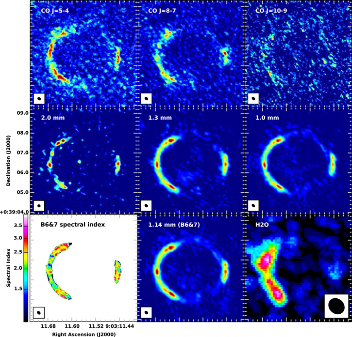
This tutorial uses the Band 6 CO data from the ALMA long baseline Science Verification observations of SDP.81, based on the initial data reduction scripts.

The CO J= 8-7 lie has a rest frequency of 921.799GHz. SDP.81 is at z=3.042, and is expected to have a width DVel of about 800 km/s.

Hopefully you can write your own CASA script, but some of the more important task inputs are given at the end of this page - only consult them if really stuck.

Overview

Subdirectory SDP81_Band6_ReferenceImages contains the original line and continuum image products:

SDP81_9exec.co87.R1uvtaper1000klambda.fits
SDP81_9exec.co87.R1uvtaper1000klambda.mom0.2sigma.fits
SDP81_9exec.h2o.R1uvtaper1000klambda.10.5kms.fits
SDP81_band6_9exec.contR1.image.fits

SDP81_Band6_CalibratedData contains

SDP81_band6_9exec.ms.co87

The calibration derived from instrumental measurements and calibration sources has been applied and the spw containing the CO line has been split out.

Examine the data

List the contents of the dataset, and note the frequency set-up.

#Chans Frame Ch0(MHz)    ChanWid(kHz) TotBW(kHz) CtrFreq(MHz) BBC Num Corrs
128   TOPO  228992.188   -15625.000   2000000.0  228000.0000     4    XX  YY

Use plotms to plot amplitude against channel (average in time). No obvious line, but there seems to be some bad data. Plot amplitude v. scan, averaging all channels and all times within a scan. You will see different noise levels corresponding to the conditions on the different days when the data were observed, but this taken care of by the weights, which include the inverse of Tsys (you can plot these if you have time). However, there are other discrepant points. Use Mark and Locate to identify the scans and antennas or baselines.

Write flagdata commands for the most obvious bad data (but no need to be too pernickety for this tutorial). Make a back-up first with flagmanager. There is a crib below, if you are stuck

Subtract the continuum

Since the line is hard to spot, esitmate the line channels using prior knowledge. From the known redshift z and rest frequency f0 (see above), the observing frequency f is given by


f=f0/(z+1) 

= 921.79970/4.042
= 228.05534

(ignoring the more subtle cosmological effects).

Use the listobs output to work out what channel corresponds to f and the total number of channels covering the line (each channel width is df). Use the radio convention, i.e. DVel=c*Df/f where Df is the frequency span corresponding to DVel. All in GHz/km/s:

f_Ch0=228.992188
df=-0.015625
DVel = 800.
Line centre channel = 0+ (f-f_Ch0)/df
c=2.998e5
Df =  (DVel/c)*f = 0.608553
Number channels across the line= Df/df

giving the line peak in channel 60 and a total line span of 39 channels (to the nearest channel).

Use uvcontsub to subtract the continuum. Set fitspw to the continuum selection of channels (help par.spw gives the syntax for specifying multiple channel ranges). Use a first-order fitorder, everything else can be default apart from the input name.

Image the line cube

The SV team found that the best line image needed a tapered beam, that is, the longest baselines are weighted down to increase the synthesised beam size and thus improve surface brightness sensitivity. Plot amplitude v. uvdistance for the file you have just created, SDP81_band6_9exec.ms.co87.contsub (average all channels, all times) and note the maximum baseline uvmax. This gives the maximum natural synthesised beam and for best results the imaging pixel size should be about 3 pixels across the beam. Since due to the tapering, the actual beam size is much larger, two pixels across the natural beam should suffice.

uvmax = 15500 metres
wavelength = c/f = 2.998e8/ 228.05534e9
beamsize=3600.*degrees(wavelength/uvmax)

This gives a natural beamsize of 17.5 mas, so we will use a pixel size of 8 mas.

Inspect the sample image of the continuum, SDP81_Band6_ReferenceImages/SDP81_band6_9exec.contR1.image.fits in the viewer. The continuum image is slightly off-centre, so we can economise on the size of the cube by centring it more precisely. Estimate the RA and Dec of the centre of the ring, and the total angular size. The gas might be more extended than the continuum, say angular size of 6 arcsec, and with an additional allowance to avoid deconvolution errors, 1024 x 8 mas pixels should be plenty. You can check that this is well within the primary beam FWHM.

tclean is a new version of clean which is somewhat faster and mroe stable, but not yet perfectly documented. Here are the important inputs, some of them you need to fill in. The original example used the observed frequency as rest frequency, so that the output velocities were centred on zero with the observed frame channel width.

os.system('rm -rf SDP81_band6_co87.clean*')
tclean(vis='SDP81_band6_9exec.ms.co87.contsub',
       imagename='SDP81_band6_co87.clean',
       specmode='cube',
       outframe='bary',          # or lsrk if you prefer
       restfreq='921.79970GHz',  # could alternatively use observed frequency
       start=**,nchan=**,        # enter relevant numbers 
       deconvolver='multiscale', # finds groups of clean components if appropriate
       scales=[0,5,15],
       imsize=**,cell='**',      # enter relevant numbers 
       uvtaper='1000klambda',    # downweight long baselines
       weighting='briggs', robust=1.0,
       phasecenter='**',         # see help for format 
       interactive=T,
       niter=50000,threshold='0.2mJy')

Once the Viewer appears:

Try opening the continuum image as contours for a guide for masking (then close it when you have made the mask)
For speed, select All Channels when masking. Draw a circle round the continuum, then change to Erase and remove the centre.
After the first hundred iterations, inspect the brightest channels and adjust the mask (set back to Add!) as required.
After one or two sets of 100 iterations, I tried setting a large mask (no holes) and changed iterations per cycle to 1000.

Image analysis

You can perform a nubmer of operations either in the viwer or using tasks; the tasks to look at are imstat, immoments and impv

General long baseline and spectral line considerations

**ALMA approx. b/w and time smearing**

Long baselines

Make sure that any antenna position corrections are applied in initial calibration
Avoid bandwidth and time smearing (see Fig.)
Choice of calibrators - need to be within 3-4 degrees, compact/modellable, bright enough to give good SNR in 15-30s (often do a check prior to observations).
Phase errors may be worse on longest baselines, less accurate phase transfer from phase-ref. Initial dynamic range may only be 50-100 even for a bright source - but if you do reach this, the source will be bright enough to self-calibrate!

Spectral Line

Check the velocity convention and reference frame - don't trust SIMBAD or NED blindly!
More time is needed for bandpass calibration in narrow channels (although errors are mostly on at least 20 MHz scales, averaging possible).
If spectral windows are much less than 2 GHz:

May need to increase calibration solution intervals in time/frequency
May need to transfer time-dependent calibration from wider to narrower spw (use bandpass cal to compensate for phase offsets)

Spectral line imaging

Identify line and continuum as far as possible from visibilities (if necessary restrict uv range, apply a shift...) or prior knowledge
If some channels are very narrow, split out averaging each spw to a coarse resolution (e.g. TDM) and estimate line-free selection for new channelisation.
Image continuum, self-calibrate if bright enough
If line is brightest, and you want to self-calibrate on a line, you need first to adjust all the data to a common rest frame (mstransform).
Either way, if you have self-calibrated, apply calibration to all data.
Subtract continuum (unless peak is much less than rms of line channels)
Image cube (maybe test a few channels first)

Crib sheet for CASA inputs

Initial flagging

These are the flags I made (there may be more small amounts of bad data, but no need to spend a long time on finding these for this tutorial). Make a back-up first with flagmanager.

flagmanager(vis='SDP81_band6_9exec.ms.co87',
         mode='save', versionname='before_moreflags')
flagdata(vis='SDP81_band6_9exec.ms.co87',
         mode='manual', scan='163', flagbackup=False)
flagdata(vis='SDP81_band6_9exec.ms.co87',
         mode='manual', scan='280~415', 
         antenna='DA49&PM04',flagbackup=False)
flagdata(vis='SDP81_band6_9exec.ms.co87',
         mode='manual', scan='349~415', 
         antenna='DA65&PM04',flagbackup=False)

Subtracting the continuum

uvcontsub(vis='SDP81_band6_9exec.ms.co87',
          fitorder=1,fitspw='0:0~40;80~127')

Imaging

You may choose different frames, values etc.

os.system('rm -rf SDP81_band6_co87.clean*')
tclean(vis='SDP81_band6_9exec.ms.co87.contsub',
       imagename='SDP81_band6_co87.clean',
       specmode='cube',
       outframe='bary',          
       restfreq='921.79970GHz',  
       start=40,nchan=40,        
       deconvolver='multiscale', 
       scales=[0,5,15],
       imsize=1024,cell='0.008', 
       uvtaper='1000klambda',    
       weighting='briggs', robust=1.0,
       phasecenter='J2000 09h03m11.555 00d39m06.43',  
       interactive=T,
       niter=50000,threshold='0.2mJy')