The ALMA Observation Support Tool (OST) is an ALMA simulator which is interacted with solely via a standard web browser. It is aimed at users who are not experts in interferometry and do not wish to familarise themselves with the simulation components of a data reduction package. It has been designed to offer full imaging simulation capability for an arbitrary ALMA observation while maintaining the accessibility of other online tools such as the ALMA Sensitivity Calculator.
Simulation jobs are defined by selecting and entering options on a standard web form. The user can specify the standard parameters that would need to be considered for an ALMA observation (e.g. pointing direction, frequency set up, duration), and there is also the option to upload arbitrary sky models in FITS format.
Once submitted the job is placed in a queue on the server running a CASA-based back-end system which processes the jobs chronologically. The user is notified by email when the job is complete.
OST Acknowledgement
A paper detailing the OST is now a now available on arXiv (arxiv.org/abs/1106.316, ADS link). The paper is to appear in the proceedings of Astronomy with Megastructures: Joint Science with the E-ELT and SKA. This is the recommended article for use when referencing the ALMA OST.
Simulation Options on the Web
Interface
This section offers a section-by-section, option-by-option
overview of the web interface, how the various options relate to the
set-up of the simulation, and occasionally going into detail about
any assumptions that the OST makes behind the scenes.
Instrument
Figure 1. Array Selection
The first menu on the web interface allows the user to select which array on the ALMA site they wish to simulate. Included in the menu are:
All Cycle 4, 5, 6, 7, 8, 9 array configurations
All Cycle 3 array configurations (plus options to do ALMA Cycle 3 + ACA simulations, where available)
All Cycle 2 array configurations (plus options to do ALMA Cycle 2 + ACA simulations)
All Cycle 1 array configurations (plus options to do ALMA Cycle 1 + ACA simulations)
Early Science (Cycle 0) array configurations (with maximum baselines of 125 m and 400 m)
An options to use the full 50-antenna ALMA.
Atacama Compact Array (ACA)
Full ALMA +ACA
About the cycle-specific options: Selecting cycle-specific configurations will simulate the capabilities of ALMA in that cycle, and therefore some observations might be restricted (you will be notified if this is the case). Please, refer to the ALMA documentation for each cycle capabilities. For this cases, the 'required resolution' options (see here) has no effect on selecting array. Instead the maximum resolution is that given by calculating the resolution using the maximum baseline. The maximum baseline is listed in the drop down menu with the exception of ALMA Early Science (Cycle 0) which are 125m compact and 400m extended.
About the full ALMA option: The simulations will be done with the full capabilities ALMA will achive in the future (e.g. observing with 50 antennas, or Band 10 Configuration 10 observations); some of these may not yet be offered in the current cycle. Although the full ALMA undergoes a continuous reconfiguration process and does not have a fixed array layout there is only a single option in the menu for this instrument. This is because the OST will select an appropriate configuration for the full array based on the subsequent resolution requirements of the simulation. There are 28 possible configurations which are consistent with those supplied within the CASA distribution and include 50 antennas. This behaviour also applies to the ALMA+ACA option.
About the User upload option:
From Version 7.0 the OST now supports user uploaded ALMA antenna configuration files. These should be in the format of a CASA '.cfg' file, but appended as a .txt file. An example is given here: .
Users are able to supply configurations containing upto 54 ALMA dishes (maximum number of 12m antenna available). The OST will only accept dishes with diameters of 7 or 12 m and not mixed configurations within a single file. Columns should be tab separated.
Users can generate their own based on their ALMA (or archival) data using the Analysis Utils casa au.buildConfigurationFile() task. This feature can be used to generate simulations which more closely match ALMA data as it was observed on the sky. To download Analysis Utils for CASA please go here:
https://casaguides.nrao.edu/index.php/Analysis_Utilities
and specfic instructions on the buildConfigurationFile() command can be found here:
https://casaguides.nrao.edu/index.php/BuildConfigurationFile ALMA+ACA simulations: This option has not been carried forward for Cycle 4 antenna configurations given the requirement for several ALMA 12-m arrays plus the ACA to cover all spatials scales for some projects. We retain the Cycle 1,2 and 3 options for historic purposes but refer the user to the ALMA Cycle 4 proposers guide for more information on combining arrays to recover different spatial scales.
When any ALMA + ACA array configuration is selected, two jobs will be run through the OST. One using the ALMA configuration and a second using the ACA configuration, (the on source time will be scaled appropriately for ACA observation). The user will therefore recieve twice the number of emails and two datasets. One results page will present the user with a link to a Python script which can be run in CASA to combine the two datasets using the CASA feather task (this script can also be found here). For ALMA Cycle 1 and Cycle 2 the ACA used is appropriate to that Early Science observing cycle. Please note that in some real Cycle 2 observations an alternate ACA configuration may be used at the discretion of the JAO, for sources with low elevation. For ALMA Cycle 2 + ACA simulations with the OST, the standard ACA configuration will always be used. The response of the Cycle 2 ACA in either configuration is similar but the uv-coverage will differ. For completness the alternate ACA configuration (7m-NS) is provided as a stand-alone option in the Cycle 2 instrument list.
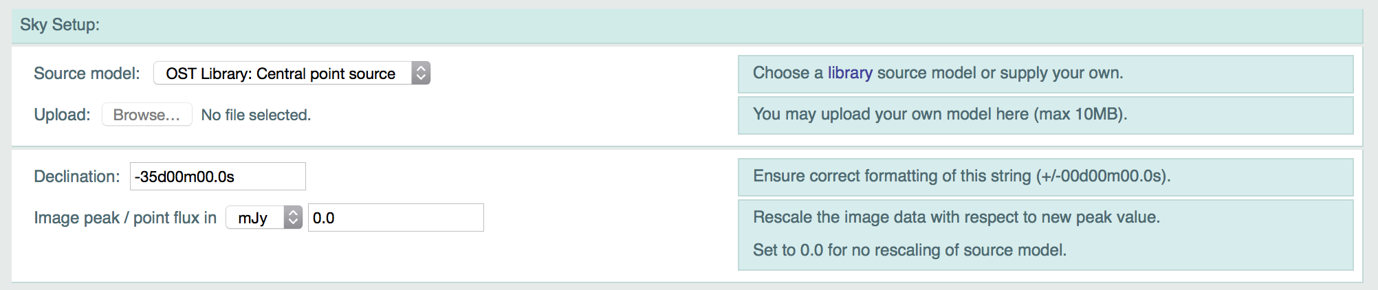
Sky Setup
Figure 2. The sky setup options on the OST front-end.
This section is where the user specifies the properties of the
source, namely its position and the ideal sky brightness
distribution that will be observed by ALMA.
Source Model
The drop-down menu in this section contains all the source models which are currently part of the OST Library. There are a variety of options here, ranging from a simple central point source to morphologically complex structures. The Library is assembled from a combination of existing observations and the results of astrophysical simulations.
The single option in this menu which does not select a pre-existing
source model is Uploaded FITS image which notifies the OST that the
user has submitted a custom sky model. There are numerous things to
consider when preparing a source model FITS file, and some hints for
this process are presented in the FITS section.
Upload a FITS file
When a user selects Uploaded FITS image from the Source Model menu, the Browse button becomes enabled. Clicking this will bring up a file
selection box and allow the user to supply an arbitrary source model
in FITS format only. Many parameters in the header of the FITS file
will be overridden by the options that the user subsequently selects
on the OST interface, however there are some parameters which must be
valid in order for the OST to process the file successfully,
specifically the angular scale of the pixels and the brightness unit
(Jy/pixel). These are discussed in the FITS section. Also, the model must have a dimension > 1 in both axes of the coordinate space (i.e., right ascension and declination).
Declination
The string in this field specifies the source Declination. It must be formatted correctly, including the leading + or - sign. The value entered here will replace the value in the header of any FITS file that is uploaded and will also be used for any source model selected from the Library.
The Right Ascension field is conspicuous by its absence. The OST does not require the user to specify this value, relying instead on the user to supply an Hour Angle value (see here) which determines the time of the observation relative to the transit time of the source.
Image Peak / Point Flux
The user can arbitrarily scale the brightness of the source
model by entering a non-zero value in this field. The original image
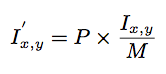
Ix,y is scaled according to:
Eqn. 1
where P is the value entered in the field and M is the original maximum value of the image. Entering a value of zero means that no image scaling will be applied. It is therefore not possible to scale an image such that all pixels are zero. The value entered in this field also controls the brightness of the point source if the user selects that particular source model. If a simulation of a pure noise field is required then this can be accomplished by selecting the point source model and
applying a flux of zero. There is also a small drop down menu which selects the unit of the value entered: Jy, mJy or
μJy.
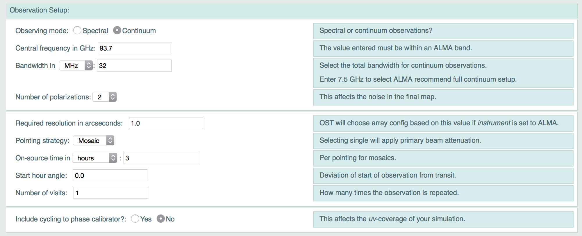
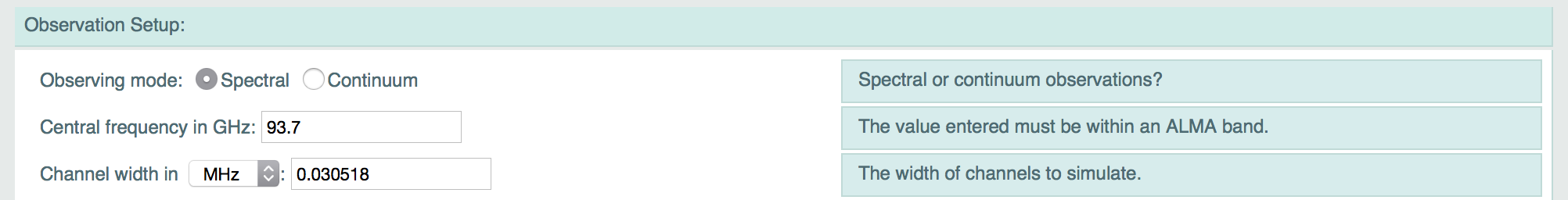
Observation Setup
Figure 3. The observation parameters the OST front-end.
This section contains options for choosing frequency setup,
observation duration, resolution considerations and a simple
mosaicking model.
Observing Mode
New for ALMA Cyle 3, the OST now offers two observing modes, Spectral or Continuum. This option allows the user to select between the two mode of OST simulation. The associated parameters for these options are discussed below.
Expected behaviours for the new Spectral mode
Creating a data cube simulation requires the user to select the option 'Spectral' for the 'Observing mode' parameter of the OST webform. If a image FITS file (i.e. one with two coordinate axis and one frequency) is uploaded (or selected from the library) with 'Observing mode' set to 'Continuum' then the OST will use the image data from the central cube channel to generate a single plane continuum simulation as in previous versions of the OST. Conversely, if 'Observing Type' = 'Spectral' is presented a FITS image with a single channel it will process it as a cube of a single channel. The OST does not add or remove spectral channels to uploaded FITS cubes.
When presented with a FITS cube and with 'Observing Type' = 'Spectral', the OST will behave as follows:
Time allocation:
As the OST is a queue based system there is a limitation on the amount of time each simulation can be allocated. To this end the OST will inspect the uploaded FITS cube, which are more computationally heavy than single plane simulations, and estimate the time required to process the simulation. The time estimate in minutes is calculated as:
Eqn. 2
where NZ is the number of channels in the cube, A(s) is a linear function based on s the larger of the two spatial dimensions (in pixels) and B(s) is a logarithmic function of s.
In previous OST versions 25 minutes has been typically been the longest a simulation has taken to run, during this time there have been few instances that the OST queue became sufficiently large that it became problematic for users. As such we limit the processing of time allowed for a FITS cube to 25 minutes. If this is exceeded the simulation will not proceed and the user will be notified.
As the time allocation is based on both the largest spatial dimension and the number of spectral channels in the cube this limitation has the affect of requiring user uploaded FITS to be either “short and fat or long and thin” (e.g. 200x200x10 or 100x100x50). The output image plane size for multichannel FITS cubes is also limited to 512x512 as opposed to 2048x2048 for single plane images (see here).
Frequency Coverage:
In 'Observing Type' = 'Spectral' mode, the user is asked to input a central observing frequency and a channel width. The OST webform prevents the user from submitting simulations with channels smaller or larger than the minimum or maximum values used by the ALMA correlator. The OST will only simulate spectral cubes up to a maximum bandwidth of 1.875GHz (the maximum width an ALMA spectral window can have).
To account for this the OST does the following. Multiplies the number of channels, nchan, in the user uploaded FITS cube by the user defined channel width. If this value exceed 1.875GHz then the total bandwidth will be truncated to 1.875GHz and the channel width set to 1.875/nchan GHz.
It is also possible that the combination of central observing frequency and channel width applied to a user uploaded FITS cube will lead to part of the bandwidth spilling over the edge of an ALMA observing band. To overcome this, the OST will calculate how much the bandwidth will overspill the band edge and will adjust the users central observing frequency to make sure all channels are within the ALMA band. This functionality ensures that the number of channels in the user uploaded FITS cube and the OST simulation are the same, to avoid any difficulty in comparison between the two. Users should be aware that this the opposite behaviour to bandwidths overspilling the band edge when the OST is in Continuum mode, where the OST will simply truncate the bandwidth.
As a final note, the processing of FITS cubes is slower than single plane imaging (as detailed above). If necessary, i.e., the OST becoming very large toward the end of the Cycle 3 call for proposals we may have to temporarily suspend the processing of FITS cubes.
Continuum Observing mode
Central Frequency in GHz (Continuum Mode)
As the name implies, this is the central frequency of the
observation in GHz, which should be within the ranges of bands 3 - 10
of ALMA. The OST will return an error if the user attempts a
simulation outside these ranges.
Bandwidth
Allows user to specify the desired observational bandwith, with a drop down menu which selects the unit of the specified bandwidth. This value has an upper limit of 7.5GHz in correspondence with the actual ALMA bandwidth limit. If 7.5GHz is exceeded then the OST will not preform the simulation, instead the user will be notified via email that their bandwidth is too large. Below this limit the options available to the user depend on the bandwith value entered as described below.
For Bandwidth ≤ 1.875GHz: This is the maximum bandwidth of a single ALMA baseband, for bandwidths in this value range the user input bandwidth will be treated as one continuous bandwidth centred around the input central frequency.
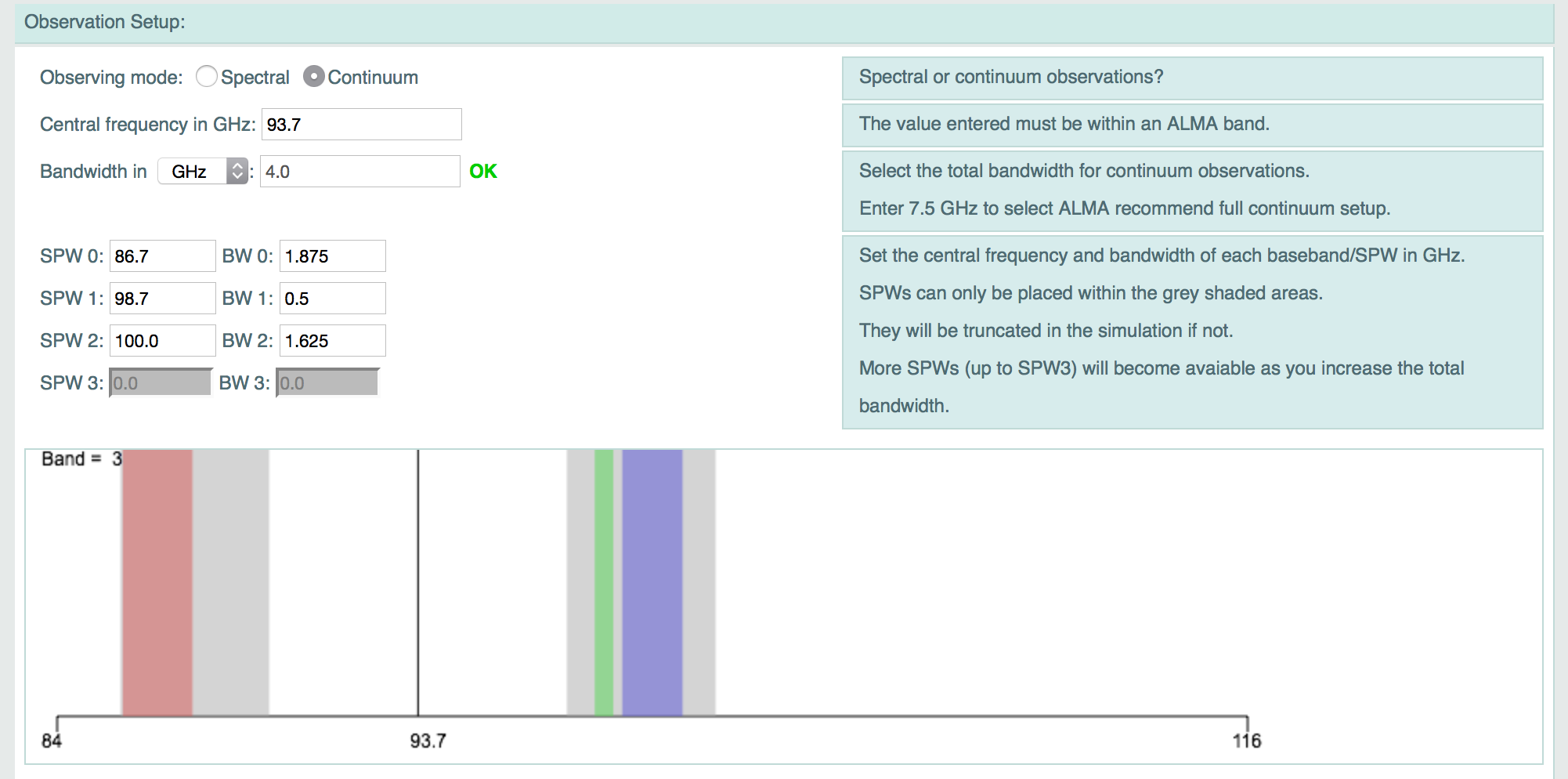
For Bandwidth > 1.875GHz and ≤ 7.5GHz: Here the user input bandwidth exceeds the maximum width of a single ALMA baseband, as such additional options will be revealed. These are the SPW 0-3 and BW 0-3 inputs, representing 4 "spectral windows" central frequencies and their associated bandwidths (in GHz). A graphic is also displayed allowing the user to places these "spectral windows" within the frequency ranges the ALMA correlator allows (based on the input Central Frequency), these are indicated by the two grey areas on the graphic. All spectral windows should be positioned within these areas. SPWs which overhang the edges of these areas will be truncated during simulation.
Depending on the users input Bandwidth the number of SPWx and BWx input boxes which are greyed out will change, by factors of n times 1.875GHz. So for Bandwidth > 1.875GHz SPW0 and 1 are available, for Bandwidth > 3.75GHz SPW0,1, and 2 are available and for Bandwidth >5.625 (and less than 7.5GHz) SPW0, 1, 2 and 3 are available.
Note: that in actual ALMA observations a greater number of spectral windows is available. We contrain the number in the OST to four to keep simulation processing times low and the OST interface as simple as possible. Figure 4a. The continuum bandwidth setup options for Bandwidth > 1.875GHz and ≤ 7.5GHz
The OST will check that the sum of the "spectral window" bandwidths specified for each of the optional BW0-3 does not exceed the user specificed total Bandwidth.
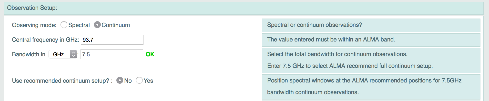
For Bandwidth = 7.5GHz: Here the user input bandwidth is the maximum bandwidth allowed by ALMA (7.5GHz). Here users will then be presented with the option to use the ALMA recommended spectral window setup for full continuum observing. This is a simple yes/no option to use the recommended frequency positions for continuum observations as specified by ALMA and the OT. Please see the ALMA Cycle 3 Technical Handbook and Proposers Guides for more information.
Figure 4b. The continuum bandwidth setup options for Bandwidth = 7.5GHz.
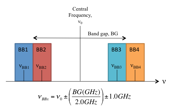
The users bandwidth will be split into 4 equally wide spectral windows of 1.875GHz. The position of these windows will then be the ALMA recommended positions if user selects Use recommended continuum setup? = yes, or positioned in both an upper and lower side band (USB and LSB) as shown in Figure 4 based on the user input central frequency. The centres of the USB and LSB are at 0.5 x the band gap for each reciever. The band gaps for different ALMA bands are present in the ALMA Technical Handbook. The central frequency position for each baseband is given by the equation also seen in Figure 4. The noise considerations are then based on the noise over each frequency range in each base band as would be done for a single continous continuum bandwidth.
Figure 5. Bandwith Setup for user input bandwidth = 7.5GHz.
If the combination of the central frequency and bandwidth (in any scenario detailed above) causes the requested frequency range to exceed the limits of an ALMA band then the OST will automatically truncate the bandwidth (and adjust the noise accordingly). If such a liberty is taken then the user will be notified.
Using Stokes Cubes
In the OST version 4 the user is presented with the option to 'Use full Stokes parameters', which is a simple yes/no option. This option can be used if (and only if) the users uploaded FITS file contains a Stokes axis, with size greater than 1, (e.g. contains Stokes I, Q, U or I, Q, U and V planes).The expected behavouir of this new feature is as follows:
If the uploaded FITS contains such a Stokes axis and the user selects 'yes' then the OST will output an image cube with the same number and types of Stokes planes as the input image.
If the uploaded FITS contains such a Stokes axis and the user selects 'no' then the OST will simple use the first Stokes axis (usually I), in the same way it would use the first frequency plane of an uploaded spectral cube.
If the user uploads a cube with both a Stokes and Frequency axis greater than 1 plane in each dimension then the OST will follow the above behaviours (depending on the yes/no option selected) but simulate just the central frequency plane of each Stokes axis.
This option is not available in spectral observing mode. For further information on this feature see the note on enhanced polarization products below.
Spectral Observing mode
Central Frequency in GHz (Spectral Mode)
As the name implies, this is the central frequency of the
observation in GHz, which should be within the ranges of bands 3 - 10
of ALMA. The OST will return an error if the user attempts a
simulation outside these ranges.
Channel width
This allows users to specify the channel width of the individual channels in their simulation. There is a drop down menu to specify the units.
Figure 6. The observation parameters the OST front-end.
Number of Polarizations
The receivers of ALMA record two orthogonal polarizations from
the incoming electromagnetic wave. By averaging both of these when
producing a map the signal to noise ratio may be improved by a factor
of sqrt(2). The OST now handles user uploaded Stokes cubes, if this is the case
then this parameter, for the puroposes of improving the noise is ignored.
Further Polarization Products
As of version 4 the OST now offers simulations of Stokes cubes with I, Q, U and V planes, in continuum mode.
For an explaination of how to simulate the with a Stokes cube please refer to this section of the OST help.
This facility is available to show the effects of ALMA sampling on the separate I, Q, U and V planes, however users should be aware that the OST does not add instrumental leakage into the simulated data. The reason for this being that the underlying CASA software upon which the ALMA OST (and indeed
Simobserve) are based does not fully handle simulations including instrumental leakage. As and when the enhanced CASA
simulation tools introduce the capability for simulations with instrumental leakage they will be implemented into the OST.
Required Resolution in arcseconds
If the user has selected ALMA in the instrument option then the value entered here will be considered, together with the frequency requirements, to select an appropriate ALMA configuration.
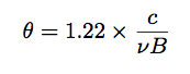
The maximum resolution θ (in radians) of an interferometer is
approximately determined by:
Eqn. 3
where c is the speed of light, ν is the observing
frequency in Hertz and B is the longest projected baseline in
metres. This equation is used to convert the required resolution into
a baseline requirement, which is then matched to the longest baseline
within the the 28 potential array layouts. Note that in practice the
resolution of an image rarely matches that of the longest baseline, as
the visibility measurements are generally weighted according to their local density in the uv-plane. Since there are always more short baselines than long ones the practical resolution is generally less than the theoretical maximum.
Remember: For all other Array options (ALMA Cycle 0, 1, and 2 and ACA) this option is ignored and instead the resolution is determined by the maximum baseline of the selected array.
Pointing Strategy for Version 5
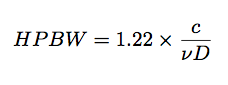
There are three options in this menu: single, mosaic and User Pointing. The field-of-view of a dish-based interferometer is a function of the diameter of the receiving elements D and the observing frequency ν. It is related to a function called the primary beam which effectively dictates the sensitivity of the instrument as a function of angle. The sensitivity is maximum at the pointing centre and tapers off for off-axis directions. A rough estimate of the half-power level of this function for a parabolic antenna such as the type that ALMA uses is:
Eqn. 4
i.e. HPBW (half-power beam width) is the number of radians away from the pointing centre at which the gain of the array drops to 0.5.
Since ALMA operates at high frequencies its field of view is
correspondingly smaller than centimetre-wave instruments with
equivalent dish sizes. As such, mosaicked observations are likely to
be necessary. These consists of many individual pointings which are
overlapped in such a way that when combined they can cover a large
area of sky with approximately uniform sensitivity.
The single option in this menu will therefore simulate a single pointing, i.e. the sky brightness will be attenuated by a model of the primary beam away from the pointing centre. The RMS noise in the final image will be related to 1/sqrt(On-source Time) as all on source time will have been spent on this single pointing.
The mosaic option will simply examine the sky area which
is to be simulated and return an approximate number of pointings,
based on a traditional hexagonal mosaic pattern, that would be needed
to cover the entire field with the required sensitivity. In effect this acts as if each pointing has been observed for the user specified on source time, so the RMS noise in the final image will be related to 1/sqrt(On-source Time).
New for version 5: The User pointing option gives the User an option to upload a pointing file. This should be in the CASA format (see example below). The OST will then image the simulation as a mosaic at the user uploaded poiting positions. The as the OST does not use Right Ascension information the pointings will be modified to alter the RA values to have the centre of the mosaic at an hour angle of 00h00m00.00s (as per Start Hour Angle). Currently there is a limit of 30 pointing positions in an uploaded pointing file, though this may be altered. Unlike the previous two options, the noise in the final image using the User pointing option is related to 1/sqrt(On-source Time/number of pointings) as the total on source time is split between the pointings.
For example, with Pointing strategy = User pointing for 7 pointings and on source time = 3 hours will result in each pointing observed for 3/7 hours and an RMS noise per pointing of 1/sqrt(3/7hours)*, whereas for Pointing strategy = mosaic for 7 pointings and on source time = 3 hours, each pointing will have an RMS noise of ~1/sqrt(3hours). * For a user uploaded mosaic where pointings result in an overlap of the ALMA primary beam the noise in the final image will be better than this due to the overlap.
Example OST/CASA pointing file:
The OST will accept User uploaded pointing files which follow the CASA ptg.txt format. Please note:
The different delimiters between numerical values for RA and Dec (: and . respectively)
This field specifies the duration of the observation, the units of which can be specified in the drop down menu. The maximum time that can be entered is 24 hours.
Start Hour Angle
This value specifies the relationship between the start of the
observation and the source transit. Acceptable values are in the range
-12 to 12 hours. For example, if the user wishes to simulate a
two-hour observation with the source transiting in the middle then the
start hour angle needs to be set to -1.
Number of visits
If the user wishes to simulate either an observation that is longer than 24 hours, or a long observation which occupies a limited range of hour angles then this field can be changed to a value other than 1.
For example, a 100-day observation can be simulated by specifying a 24-hour track in the on-source time field, and entering 100 in the number of visits field.
Similarly, if there are strict hour angle requirements, e.g. only an hour angle range of +/-2 is acceptable but the user wishes to simulate 20 hours of observing then start hour angle should be set to -1, on-source time should be set to 2 and number of visits should be set to 10.
It is worth bearing in mind when considering this option and the previous two that for certain Declination and hour angle combinations the source may well be below the horizon. The OST recognises that the Earth is opaque, and will naturally not consider such scans when calculating the noise in the map. It will however warn the user that the observing time that was requested has been shortened, and that the on-source time that was achieved may be at odds with what was requested.
Include cycling to phase calibrator?
This yes/no option is used to toggle the ability to include in the simulation time off source, where in true observations a phase calibrator would be observed. If set to 'no' then the on source time is treated as a single block of on source time. If set to 'yes' the user is presented the following options:
Phase Cycle
A new option since ALMA Cycle 1, this field specifies the on source time between cuts to a hypothetical phase calibrator
to better simulate the uv-coverage of a simulation. The OST does NOT create a phase calibration simulation to
accompany your simulation, this is simply a time parameter for sectioning up the on source time. The phase cycle is limited to between 300 and 600 seconds
(5 and 10 minutes) which are typical values for ALMA observations.
On Phase
A new option for ALMA Cycle 1, this field specifies the time spent on a hypothetical phase calibrator at the end of each
on source cut (as specified by the Phase Cycle time see above). Again the OST does NOT create a phase calibration
simulation to accompany your simulation, this field is simply a time parameter for separating the on source time cuts. The on phase time is limited to between 30 and 120 seconds
(0.5 and 2.0 minutes) which are typical values for ALMA observations.
Corruption - atmospheric conditions
Figure 7. Corruption Control.
Artefacts in an interferometric image derived from a genuine observation origin due to a variety of effects, including calibration errors, atmospheric effects and the thermal conditions of the receivers. Even in the case of a perfect observation, the latter is something that cannot be mitigated. The thermal noise introduced by the system temperature is the absolute noise-floor in an interferometric map below which sources cannot be detected.
Many things contribute to the system temperature. The two major unwanted sources for ALMA are the temperature of the receivers themselves (Trec) (which are cryogenically cooled in order to minimise their contribution), and the sky temperature (Tsky) Even at the high and dry site at which ALMA is built the effects of the water vapour in the atmosphere can still be significant.
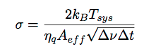
The RMS of the noise perturbation to the visibility, that is the single complex number which is the per-polarization, per-channel correlation product of a pair of antennas, is given in units of Janskys by:
Eqn. 5
where kB is the Boltzmann constant, Tsys
= Trec + Tsky is the system
temperature in K, ηq = 0.9 and is an
efficiency term associated with digitization losses during
correlation, Aeff = ηa
× Ageom is the effective area in m2, equal to the aperture efficiency (assumed to be 0.9) multiplied by the geometric area of a single antenna, Δν is the channel bandwidth in Hz and Δt is the integration time per visibility in seconds.
The receiver temperatures are fixed per-band. is derived from a model of the atmospheric transparency at the ALMA site via:Eqn. 6
where Tatmos is the atmospheric temperature (assumed to be 260 K) and γ is the transmission fraction.
The single menu option in the Corruption section relates to
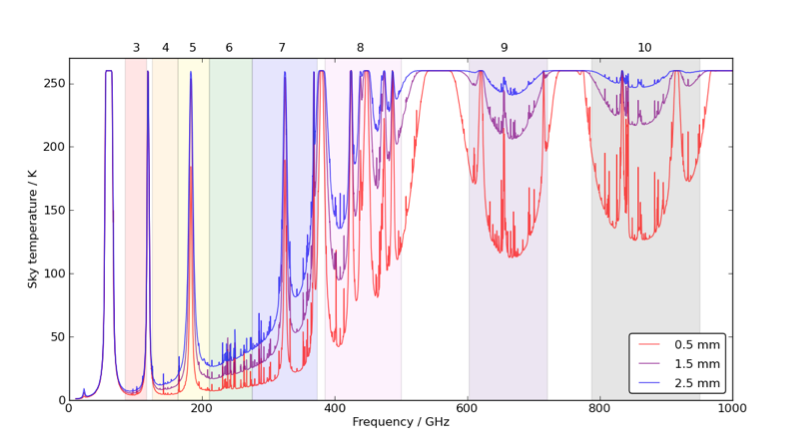
seven levels (octiles) of precipitable water vapour (PWV): 0.472, 0.658, 0.913, 1.262, 1.796, 2.748 and 5.186 mm, corresponding to the PWV values of the ALMA Sensitivity Calculator. The atmospheric transmission fraction as a function of frequency for three of these levels is shown in Figure 8. The corresponding atmospheric temperature profiles are shown in Figure 9.
Figure 8. Atmospheric transmission fraction at the ALMA site
asa functionof frequency for three column densities of percipitable
water vapour.
Interpolative functions are fitted to these plots so that the
transparency can be derived for arbitrary frequencies and the
corresponding sky temperature can be calculated via Equation 5 for
the selected level of PWV. To account for the variation of
Tsky within large bandwidths, the values are
calculated at ten points across the band and an average is taken. This value is then added to Trec to form
Tsys for use in Equation 4.
Figure 9. Sky temperature at the ALMA site as a function of
frequency for three column densities of precipitable water vapour,
with an assumed atmospheric temperature of 260K.
Imaging
Figure 10. The imaging options on the OST front-end.
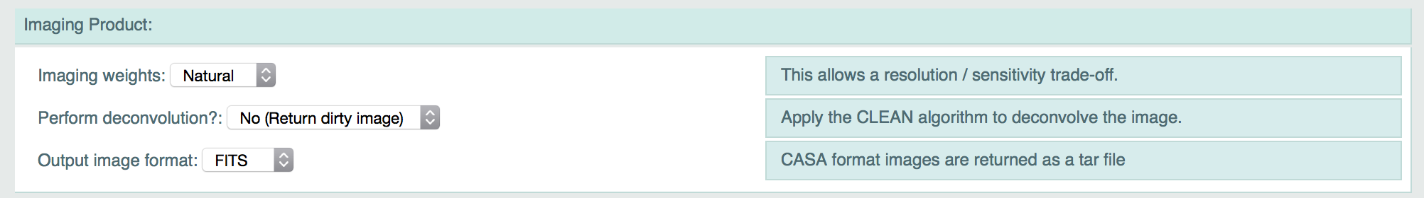
Imaging weights
As mentioned previously, the visibilities are gridded and weighted, prior to being Fourier transformed into a map. There are generally two extremes of weighting function. Natural weighting means the visibilities are weighted according to the number of measurements within a given region of the uv-plane. As there is a higher density of points around the centre of the uv-plane, which is occupied by the shortest baselines, the longest baselines which provide the highest resolution are downweighted. This weighting scheme provides the maximum sensitivity, but the resolution will be lower than that offered by the longest baselines.
Uniform weighting as the name suggests applies equal weighting to all visibilities, and offers the maximum resolution.
Briggs' (1995) weighting scheme represents an intermediate approach. Tuning of a parameter known as robustness results in a sliding trade-off between uniform and natural weighting. The OST offers only the central value.
Preform deconvolution?
The image formed by Fourier transforming the visibilities is known as the dirty image, as it is convolved at all points with the point spread function of the array (known as the dirty beam). The shape of the dirty beam is directly coupled to the uv-coverage of the observation. Deconvolution of the dirty image within the OST is performed by the CLEAN algorithm.
The CLEAN cycle is terminated when the theoretical noise limit in the map is reached.
Output Image Format
The OST can return the simulated and optionally-deconvolved
image in either FITS format or CASA image format. If the latter is
chosen then the image will be provided in a tar file.
Your e-mail address
Figure 11. One of the most important fields on the OST web form.
The final field on the web form is for the email address of the
user. An initial confirmation email will be sent to say that the
simulation job has been submitted successfully. A subsequent email
will be sent alerting the user when the job has been processed. This
email will contain a link to a webpage which will contain either the
results of the simulation or, in the event that the simulation fails
for a reason that the OST can recognise, an error message and a hint
on how to re-submit the simulation successfully.
The Results Page
Once the simulation is complete the user will receive an email
containing a link to the results page. All images on the results
page can be clicked to bring up the image in full-resolution.
Results Overview
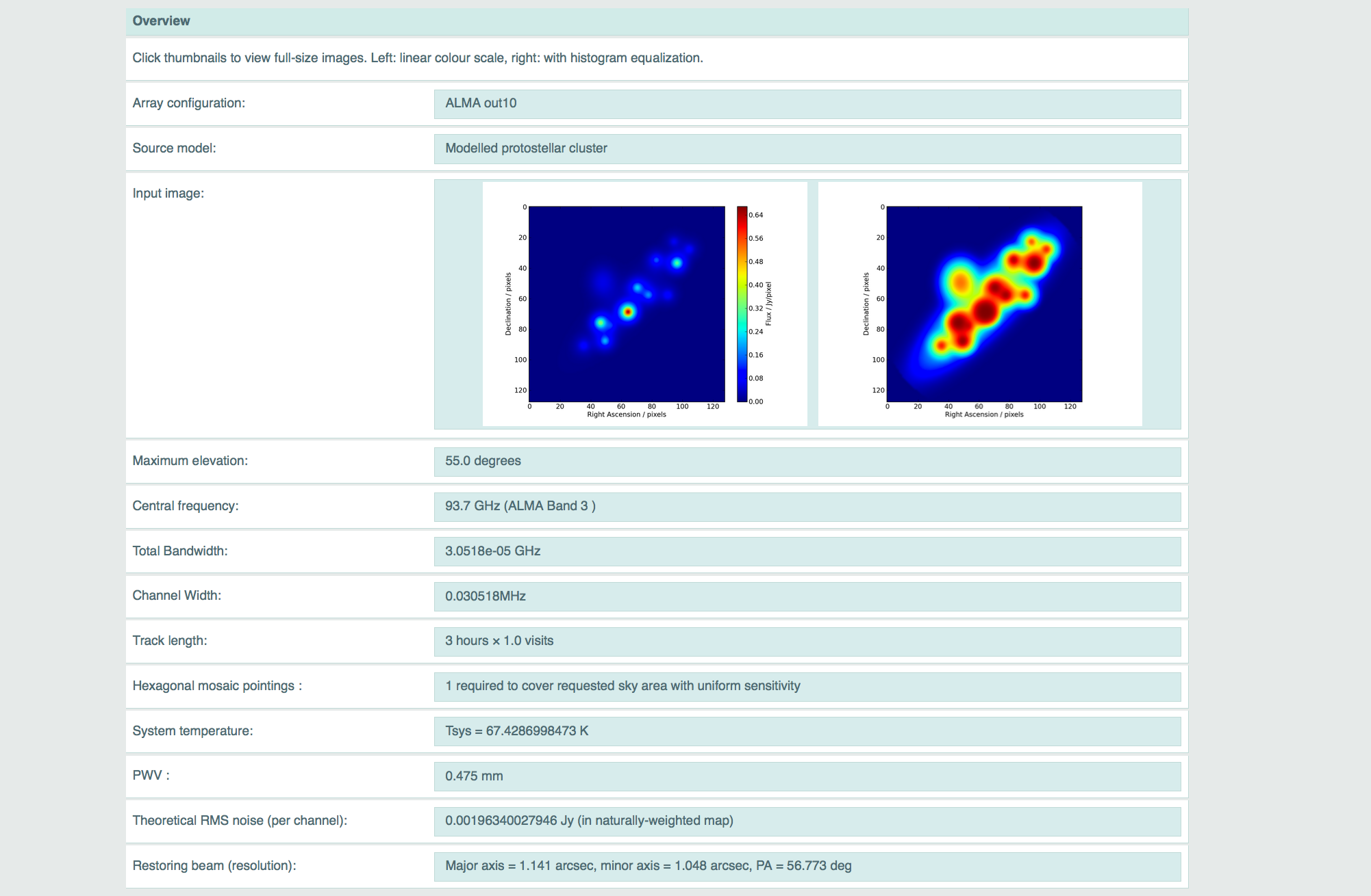
Figure 12. The Overview section of the results page.
The first section of the output page contains a few facts and figures about the simulation. Many of these simply repeat the parameters that were entered into the main OST front end, including the central frequency and bandwidth, the on-source time and the level of precipitable water vapour that was selected in the corruption section.
The array configuration field will echo the instrument which was selected by the user, although in the case of simulations performed based on the full ALMA array it will also return the out configuration which was chosen by the OST based on the resolution requirements.
Other parameters are derived from the outcome of the simulation itself. The theoretically-calculated RMS noise in an appropriately-weighted map is presented, which provides an immediate value for checking against RMS values measured from the simulated map itself.
The size (major- and minor-axis and position angle) of a two-dimensional Gaussian fitted to the central lobe of the PSF is also returned. This is essentially the resolution of the simulated observation. This Gaussian is also used as the restoring beam during deconvolution.
If the user has uploaded a FITS file or selected a non-point-source model from the OST library then the overview section will also contain two thumbnail images of the input model.
Histogram Equalization
When a sky image is rendered to appear on the results page it is done so with two different pixel intensity transfer functions. The image on the left will be a linear transfer function whereby the colour map is applied linearly to pixel values which ra0nge from zero to the maximum value in the image.
The image on the right will have been treated with an image processing
technique known as histogram equalization. Histogram equalization is an image processing technique which adjusts the pixel intensity histogram of an image such that it has a flat distribution. This is particularly useful for enhancing low level structure in images where the dynamic range is governed by a few very bright pixels.
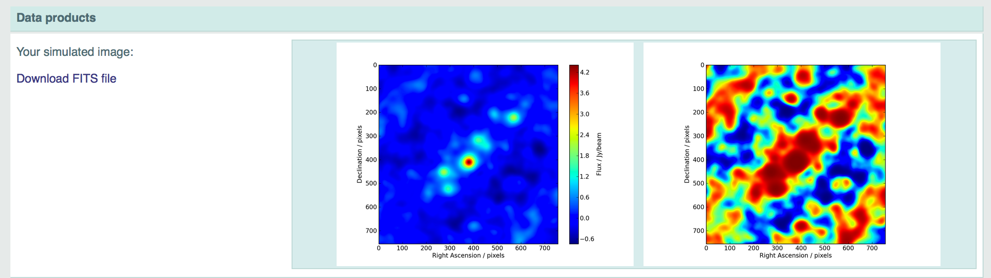
Your Simulate Image
Figure 13. Thumbnail images of the final simulated image with
the FITS file download link on the left.
This section presents two thumbnails showing the final image (either the dirty image or the deconvolved image, depending on what was requested) with and without histogram equalization. In the left-hand column there is also a link to either the FITS file or the tar file containing the CASA format image.
Note that some browsers may attempt to render the FITS image, so it is
recommended that this link is right-clicked, and the file is saved to
disk manually.
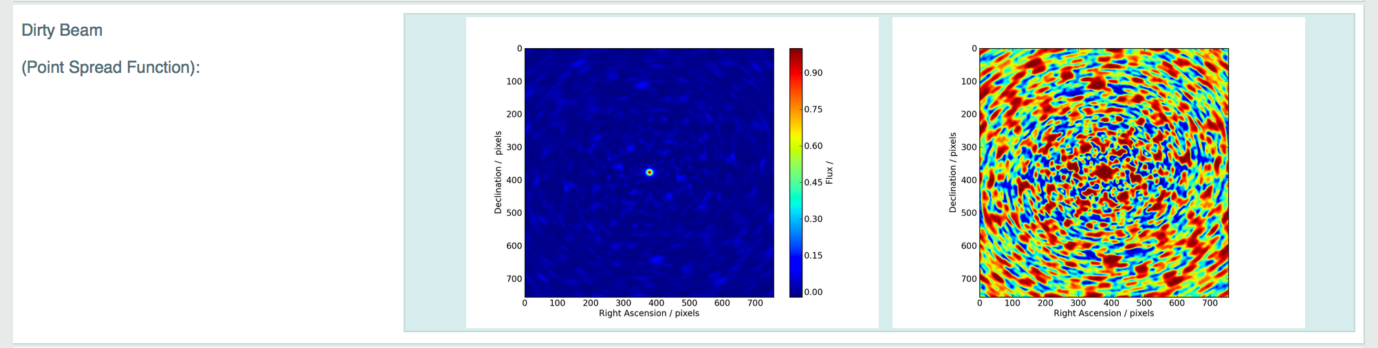
Dirty Beam (point-spread function)
Figure 14. Thumbnail images of the dirty beam (point-spread function).
The pair of images in this section show the dirty beam, or array point spread function, on the same scale as the simulated image. The central peak of this image is the component to which a Gaussian is fitted in order to determine the parameters of the restoring beam presented in the overview section.
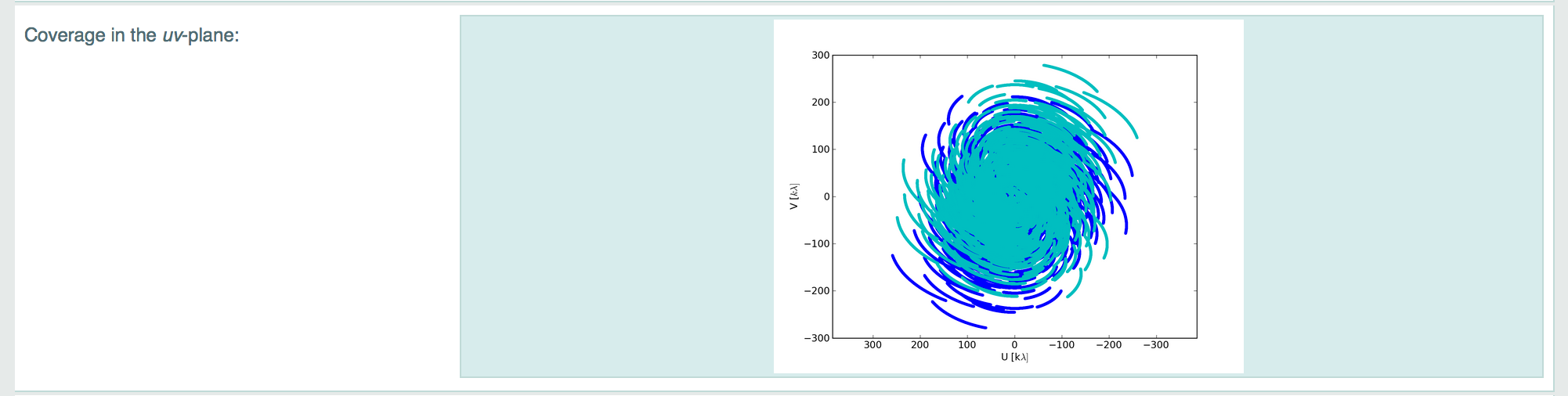
Coverage in the uv-plane
Figure 15. The uv-coverage plot.
The uv-plane coverage is determined by the layout of the antennas, hour-angle range, duration and frequency of the observation, and the declination of the source. The visibility formed by each baseline (and its complex conjugate) occupy a single point in the uv plane, representing the sampling of a single Fourier component of the sky brightness distribution. By adding more antennas, more baselines are formed and more Fourier components are measured per integration. Earth rotation changes the projection of the baselines on the sky, and further fills up the uv-plane coverage. Projected baselines also change depending on the pointing direction, thus the source elevation affects the uv-coverage.
The image presented in this section is derived directly from the uv points in the simulated measurement set.
Atmospheric Transmission
Figure 16. The atmospheric transmission again frequency for the
selected PWV levels. ALMA bands and the frequency setup of the
simulation are also shown.
The plots in this section show the atmospheric transmission fraction for the ALMA site as a function of frequency, delineated by the red line. The coloured regions on the left-hand plot correspond to bands 3 - 10 of ALMA, and these are numbered above. The right-hand plot shows a zoom-in on the specific band of the simulation. In both cases the vertical bright green line shows the frequency coverage of the simulated observation.
As mentioned in the Corruption section, the atmospheric transmission is used to derive a sky temperature for noise calculation purposes, and the red trace in these plots varies depending on the level of PWV selected in the corruption menu.
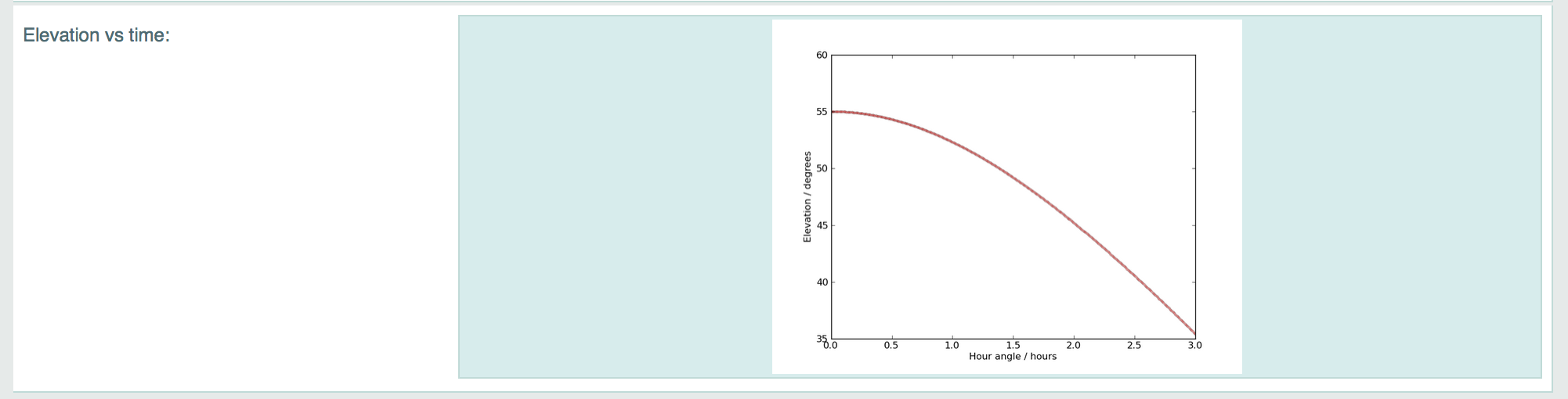
Elevation vs Time
Figure 17. Elevation again Time.
The final plot shows the elevation of the source in degrees as a function of time for the duration of the observation. If the source drops below the elevation limit (currently 8 degrees) then the red line becomes fainter. Such scans do not contribute to the final image or noise measurement for obvious reasons.
Diagnostics
Presently this section simply contains the amount of time that the server took to process the simulation job from when it was picked up from the queue to when the job complete email was sent. The time it takes to process a simulation job depends primarily on the length of the observation, the size of the image that is required, and whether or not deconvolution was requested.
Note that if an observation longer than 24 hours is requested it will not cause an increase in processing time as beyond this point the added noise is simply scaled accordingly (the Δt term in Equation 4). This is valid as at this point the full range of spatial scales is sampled due to Earth rotation, and it also serves to keep the data volumes down.
FITS Requirements
FITS Header Keywords Required by the OST.
To function correctly the OST requires certain key FITS Header keyword parameters to be present these are listed below:
BUNIT: The physical units of the FITS image array values.
CDELTn*: Coordinate increment along axis n.
CROTAn: Coordinate system rotation angle.
CUNITn: Coordinate system unit e.g. 'deg', 'Hz', etc.
CDn_n: Usually a matrix of four values which describe the mapping of the Coordinate system within the FITS image, i.e both increment and rotation. CDn_n matrix values and CDELTn and CROTAn are degenerate.
CTYPEn: Name of the CDELTn coordinate axis.
NAXIS: Number of axes.
NAXISn: Size of the axis n.
RESTFRQ: For uploaded cubes only. Rest frequency of observations.
For more information on FITS keywords please see this web page and here for more on the CDn_n matrix.
Additionally the FITS keyword BITPIX must conform to identifying float/double data type (BITPIX=-32 or -64) not integer values (BITPIX=8, 16 or 32). For examples please refer to this webpage. This is a common problem when fits files have been generated from images using the GNU Image Manipulation Program (GIMP).
An experimental Python script has been created to check FITS headers and correct BITPIX values. It is available, along with more information, here.
(* where n in an integer).
FITS Image Requirements.
File Size
Presently the maximum allowed image dimension is 2048 pixels. If a simulation job requires a larger image than this then the user is warned, but only the sky area corresponding to the central 2048 × 2048 (continuum) / 512 × 512 pixel (spectral n_chan >1) region is imaged from the simulated visibility set.
Thus the most computationally intense job that can be submitted to the server would be a 24-hour observation requiring the imaging and deconvolution of a 2048 × 2048 pixel image. Such a job would typically keep the server busy for around 15 minutes.
On the other hand, the image must have a dimension > 1 in both axes of the coordinate space (i.e., right ascension and declination). For example, images 500 × 1 (or 1 × 500) cannot be processed.
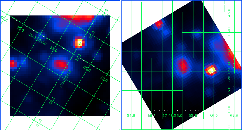
Rotation
Many astronomical instruments provide image files in which the 'x' and 'y' coordinate axes are not orientated with equatorial north corresponding to 'up' (and east == 'left'). For example see Figure 18.
Figure 18. Example of rotated image, Left: Image with orientated by pixel axis. Right: Image rotated such that equatorial north corresponding to 'up' (and east == 'left').
The OST does not rotate images, instead it assumes that an uploaded image does have equatorial north corresponding to 'up'. This may affect the representative nature of the output simulations for uploaded sky images which are rotated away from north== up by greater than ~30 degrees. This affect will be particularly pronounced in simulated observations at high and low declinations for sources which have extended emission in E-W directions as the synthesised beam will be elongated N-S.
As ALMA moves toward full science the orientation of an uploaded image for simulation will become less problematic as the beam will tend to be near round but this affect should be taken into account whenever you are using the OST for simulating images.
Fits images can be rotated prior to their use with the OST using e.g. PyFits, AstroPy, IDL, STARLINK etc.
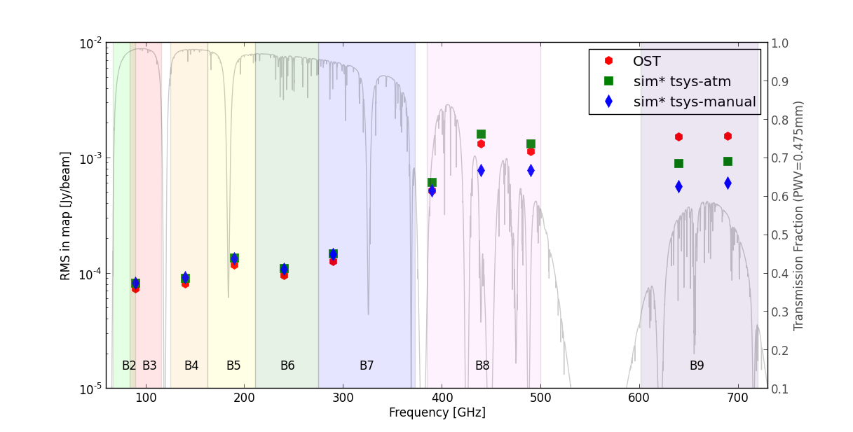
Figure 19 presents a comparison of the rms noise (in Jy/beam) as calcuated for empty field images (i.e. blank input images with 0 emission across the whole image). It can be seen that between ALMA bands 3 to 7 the noises compare well. Through Band 8 and all of Band 9 the noise comparison shows some divergence, this is attributable to the how the noise is calculated differently between the OST and simobserve. Ultimately, noise estimates for ALMA proposals should be taken solely from the ALMA sensitivity calculator (ASC) and not from simulations produced by the OST or simobserve. A comparison with the ASC is forthcoming.
Figure 19. Noise Comparison.
Figure 19 compares the noise values assumed by the OST with those
used in the two Tsys modes.


 Eqn. 1
where P is the value entered in the field and M is the original maximum value of the image. Entering a value of zero means that no image scaling will be applied. It is therefore not possible to scale an image such that all pixels are zero. The value entered in this field also controls the brightness of the point source if the user selects that particular source model. If a simulation of a pure noise field is required then this can be accomplished by selecting the point source model and
applying a flux of zero. There is also a small drop down menu which selects the unit of the value entered: Jy, mJy or
μJy.
Eqn. 1
where P is the value entered in the field and M is the original maximum value of the image. Entering a value of zero means that no image scaling will be applied. It is therefore not possible to scale an image such that all pixels are zero. The value entered in this field also controls the brightness of the point source if the user selects that particular source model. If a simulation of a pure noise field is required then this can be accomplished by selecting the point source model and
applying a flux of zero. There is also a small drop down menu which selects the unit of the value entered: Jy, mJy or
μJy.
 Eqn. 2
where NZ is the number of channels in the cube, A(s) is a linear function based on s the larger of the two spatial dimensions (in pixels) and B(s) is a logarithmic function of s.
In previous OST versions 25 minutes has been typically been the longest a simulation has taken to run, during this time there have been few instances that the OST queue became sufficiently large that it became problematic for users. As such we limit the processing of time allowed for a FITS cube to 25 minutes. If this is exceeded the simulation will not proceed and the user will be notified.
As the time allocation is based on both the largest spatial dimension and the number of spectral channels in the cube this limitation has the affect of requiring user uploaded FITS to be either “short and fat or long and thin” (e.g. 200x200x10 or 100x100x50). The output image plane size for multichannel FITS cubes is also limited to 512x512 as opposed to 2048x2048 for single plane images (see here).
Frequency Coverage:
In 'Observing Type' = 'Spectral' mode, the user is asked to input a central observing frequency and a channel width. The OST webform prevents the user from submitting simulations with channels smaller or larger than the minimum or maximum values used by the ALMA correlator. The OST will only simulate spectral cubes up to a maximum bandwidth of 1.875GHz (the maximum width an ALMA spectral window can have).
To account for this the OST does the following. Multiplies the number of channels, nchan, in the user uploaded FITS cube by the user defined channel width. If this value exceed 1.875GHz then the total bandwidth will be truncated to 1.875GHz and the channel width set to 1.875/nchan GHz.
It is also possible that the combination of central observing frequency and channel width applied to a user uploaded FITS cube will lead to part of the bandwidth spilling over the edge of an ALMA observing band. To overcome this, the OST will calculate how much the bandwidth will overspill the band edge and will adjust the users central observing frequency to make sure all channels are within the ALMA band. This functionality ensures that the number of channels in the user uploaded FITS cube and the OST simulation are the same, to avoid any difficulty in comparison between the two. Users should be aware that this the opposite behaviour to bandwidths overspilling the band edge when the OST is in Continuum mode, where the OST will simply truncate the bandwidth.
As a final note, the processing of FITS cubes is slower than single plane imaging (as detailed above). If necessary, i.e., the OST becoming very large toward the end of the Cycle 3 call for proposals we may have to temporarily suspend the processing of FITS cubes.
Eqn. 2
where NZ is the number of channels in the cube, A(s) is a linear function based on s the larger of the two spatial dimensions (in pixels) and B(s) is a logarithmic function of s.
In previous OST versions 25 minutes has been typically been the longest a simulation has taken to run, during this time there have been few instances that the OST queue became sufficiently large that it became problematic for users. As such we limit the processing of time allowed for a FITS cube to 25 minutes. If this is exceeded the simulation will not proceed and the user will be notified.
As the time allocation is based on both the largest spatial dimension and the number of spectral channels in the cube this limitation has the affect of requiring user uploaded FITS to be either “short and fat or long and thin” (e.g. 200x200x10 or 100x100x50). The output image plane size for multichannel FITS cubes is also limited to 512x512 as opposed to 2048x2048 for single plane images (see here).
Frequency Coverage:
In 'Observing Type' = 'Spectral' mode, the user is asked to input a central observing frequency and a channel width. The OST webform prevents the user from submitting simulations with channels smaller or larger than the minimum or maximum values used by the ALMA correlator. The OST will only simulate spectral cubes up to a maximum bandwidth of 1.875GHz (the maximum width an ALMA spectral window can have).
To account for this the OST does the following. Multiplies the number of channels, nchan, in the user uploaded FITS cube by the user defined channel width. If this value exceed 1.875GHz then the total bandwidth will be truncated to 1.875GHz and the channel width set to 1.875/nchan GHz.
It is also possible that the combination of central observing frequency and channel width applied to a user uploaded FITS cube will lead to part of the bandwidth spilling over the edge of an ALMA observing band. To overcome this, the OST will calculate how much the bandwidth will overspill the band edge and will adjust the users central observing frequency to make sure all channels are within the ALMA band. This functionality ensures that the number of channels in the user uploaded FITS cube and the OST simulation are the same, to avoid any difficulty in comparison between the two. Users should be aware that this the opposite behaviour to bandwidths overspilling the band edge when the OST is in Continuum mode, where the OST will simply truncate the bandwidth.
As a final note, the processing of FITS cubes is slower than single plane imaging (as detailed above). If necessary, i.e., the OST becoming very large toward the end of the Cycle 3 call for proposals we may have to temporarily suspend the processing of FITS cubes.
 Eqn. 3
where c is the speed of light, ν is the observing
frequency in Hertz and B is the longest projected baseline in
metres. This equation is used to convert the required resolution into
a baseline requirement, which is then matched to the longest baseline
within the the 28 potential array layouts. Note that in practice the
resolution of an image rarely matches that of the longest baseline, as
the visibility measurements are generally weighted according to their local density in the uv-plane. Since there are always more short baselines than long ones the practical resolution is generally less than the theoretical maximum.
Eqn. 3
where c is the speed of light, ν is the observing
frequency in Hertz and B is the longest projected baseline in
metres. This equation is used to convert the required resolution into
a baseline requirement, which is then matched to the longest baseline
within the the 28 potential array layouts. Note that in practice the
resolution of an image rarely matches that of the longest baseline, as
the visibility measurements are generally weighted according to their local density in the uv-plane. Since there are always more short baselines than long ones the practical resolution is generally less than the theoretical maximum.
 Eqn. 4
i.e. HPBW (half-power beam width) is the number of radians away from the pointing centre at which the gain of the array drops to 0.5.
Since ALMA operates at high frequencies its field of view is
correspondingly smaller than centimetre-wave instruments with
equivalent dish sizes. As such, mosaicked observations are likely to
be necessary. These consists of many individual pointings which are
overlapped in such a way that when combined they can cover a large
area of sky with approximately uniform sensitivity.
Eqn. 4
i.e. HPBW (half-power beam width) is the number of radians away from the pointing centre at which the gain of the array drops to 0.5.
Since ALMA operates at high frequencies its field of view is
correspondingly smaller than centimetre-wave instruments with
equivalent dish sizes. As such, mosaicked observations are likely to
be necessary. These consists of many individual pointings which are
overlapped in such a way that when combined they can cover a large
area of sky with approximately uniform sensitivity.

 Eqn. 5
where kB is the Boltzmann constant, Tsys
= Trec + Tsky is the system
temperature in K, ηq = 0.9 and is an
efficiency term associated with digitization losses during
correlation, Aeff = ηa
× Ageom is the effective area in m2, equal to the aperture efficiency (assumed to be 0.9) multiplied by the geometric area of a single antenna, Δν is the channel bandwidth in Hz and Δt is the integration time per visibility in seconds.
The receiver temperatures are fixed per-band. is derived from a model of the atmospheric transparency at the ALMA site via:
Eqn. 5
where kB is the Boltzmann constant, Tsys
= Trec + Tsky is the system
temperature in K, ηq = 0.9 and is an
efficiency term associated with digitization losses during
correlation, Aeff = ηa
× Ageom is the effective area in m2, equal to the aperture efficiency (assumed to be 0.9) multiplied by the geometric area of a single antenna, Δν is the channel bandwidth in Hz and Δt is the integration time per visibility in seconds.
The receiver temperatures are fixed per-band. is derived from a model of the atmospheric transparency at the ALMA site via: Eqn. 6
where Tatmos is the atmospheric temperature (assumed to be 260 K) and γ is the transmission fraction.
The single menu option in the Corruption section relates to
seven levels (octiles) of precipitable water vapour (PWV): 0.472, 0.658, 0.913, 1.262, 1.796, 2.748 and 5.186 mm, corresponding to the PWV values of the ALMA Sensitivity Calculator. The atmospheric transmission fraction as a function of frequency for three of these levels is shown in Figure 8. The corresponding atmospheric temperature profiles are shown in Figure 9.
Eqn. 6
where Tatmos is the atmospheric temperature (assumed to be 260 K) and γ is the transmission fraction.
The single menu option in the Corruption section relates to
seven levels (octiles) of precipitable water vapour (PWV): 0.472, 0.658, 0.913, 1.262, 1.796, 2.748 and 5.186 mm, corresponding to the PWV values of the ALMA Sensitivity Calculator. The atmospheric transmission fraction as a function of frequency for three of these levels is shown in Figure 8. The corresponding atmospheric temperature profiles are shown in Figure 9.